Tutorial

Mapping Humanities Data in RStudio with sf (CSV → Map → PNG)

If you have humanities data that includes locations, like sites of photos, landmarks from a project, event locations, or places tied to archival materials, you can map it quickly in RStudio using R’s spatial tools. This workflow is useful in Digital Arts & Humanities because it turns a simple spreadsheet into a reproducible map you can update anytime.

In this tutorial, I’ll show how to take a CSV with latitude/longitude, convert it into a spatial dataset using sf, plot it on a clean world (or regional) basemap from Natural Earth, label points, and export the final map as a high-quality PNG.

What you’ll produce: a map image (dh_map.png) generated directly from your data.

Step 1

Make a simple CSV

Create a file in sheets with these exact columns:

• name (what you want the label to say)
• lat (latitude)
• lon (longitude)
• optional: year, note, etc.

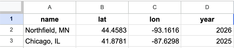
Save this sheets file as a csv and you’re done with step 1.

Step 2

Download RStudio and create a new rscript and In RStudio:
Session → Set Working Directory → Choose Directory… → select the folder (e.g., Downloads).

Run this code on your r script to confirm:

getwd()
list.files()

Step 3

Now comes the code. Paste this code and run the whole thing. What we are doing is installing/loading packages for spatial data (sf), plotting (ggplot2), reading CSVs (readr), and a basemap (rnaturalearth).

install.packages(c(
“sf”, “ggplot2”, “readr”, “dplyr”,
“rnaturalearth”, “rnaturalearthdata”,
“ggrepel”
))

library(sf)
library(ggplot2)
library(readr)
library(dplyr)
library(rnaturalearth)
library(ggrepel)

Step 4

Import your CSV into R

Run this code:

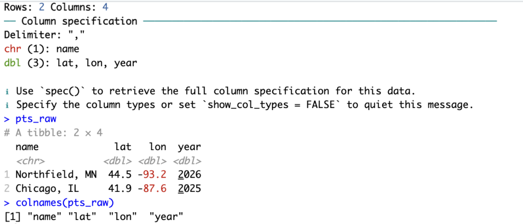
pts_raw <- read_csv(“blog – Sheet1.csv”)
pts_raw
colnames(pts_raw)

You should see your table print out and your column names listed (mine printed: "name" "lat" "lon" "year").

Step 5

Convert the CSV into a spatial object (sf)

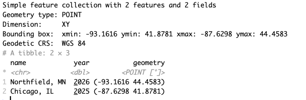
This tells R: “these rows are geographic points.”

Run this code:

pts <- pts_raw %>%
st_as_sf(coords = c(“lon”, “lat”), crs = 4326)

pts

Step 6

Load a base map

Run this:

world <- ne_countries(scale = “medium”, returnclass = “sf”)

Step 7 — Plot the map (points + labels)

Because ggrepel wasn’t available on my R version, I labeled points using extracted X/Y coordinates (this avoids extra installs and keeps it stable).

Run this:

# Extract X/Y coordinates for labeling
pts_labels <- cbind(pts_raw, st_coordinates(pts))

p <- ggplot() +
geom_sf(data = world) +
geom_sf(data = pts, size = 3) +
geom_text(
data = pts_labels,
aes(x = X, y = Y, label = name),
nudge_y = 1
) +
coord_sf(expand = FALSE) +
labs(
title = “Mapping Cities from a CSV in RStudio”,
subtitle = “Spreadsheet → sf → Map”,
caption = “Basemap: Natural Earth”
)

p

Step 7 — Export the map as a PNG for your blog post

Save the map as a high-quality image:

Run:

ggsave(“dh_map.png”, p, width = 10, height = 6, dpi = 300)

Check your folder (Downloads, if that’s your working directory). You should now see dh_map.png.

You’re Done!